Intro to Econ: Ninth Lecture – Risk Premia under Independent Risks

In the previous post we had the following problem. We were wondering about which interest rate we could expect to see for a loan for a particular risky project. You would like to get a loan, and an investor might like to give it to you. The question was, under what conditions you would get this loan, if you get it at all. Recall, that your project can turn out to be good or bad and that investors generally agree about the chances and consequences of either outcome. The problem can be summarized by the following table, where is the repayment amount that you pay back to the investor in case of the project being successful. If it is unsuccessful you pay nothing, because you have nothing. You “default” on your loan in that case. This is the risk the investor takes on when she or he gives you this loan.

 

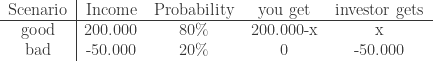
We figured out that you will not accept the loan if the repayment amount is more than € 200.000 (that would be an interest rate of 200%). Because then you have nothing to gain from this project. In reality, you might not even accept anything close to 200%, but we will come back to this problem later.

We also figured out that the investor will (almost) certainly not accept an interest rate below 12.5%, as otherwise the investor expects a negative return on their investment and would then be better off just putting her or his money under a mattress or, I guess, in a safe or vault. By the way, for a very long time the Catholic Church (and other religions) considered positive interest rates morally wrong. In such a world, you probably wouldn’t get a loan for your great project, unless you find a way around this problem. And that would probably be a shame (see previous post).

In this post I want to think about whether an investor will really accept an interest of 12.5% (or slightly above) given that the investor now takes all the risk and at an interest rate of 12.5% only expects a zero return. The answer to this question, it turns out, all depends on whether the risk in this project is essentially stochastically independent of all other risks inherent in all other projects or not.

Imagine that your investor, perhaps a bank, has a lot of money and your project is just one of many that they invest in. Assume, for simplicity, that all projects that they could invest in are just like yours, and that all risks inherent in these projects are stochastically independent of each other. This means, for instance, that if your project fails, this has no effect on the chances of other projects failing. This is not always a plausible assumption, and we will think about what happens when it is not satisfied a little further down. But if they are all independent of each other, then something magical, the law of large numbers, happens. Then investing in all of these essentially has zero risk. To see this suppose that the interest rate is 20% for all these projects. Then from each project there is a 20% chance the investor loses € 50.000 and an 80% chance the investor gains € 20.000 ().

Now I have two ways to try to convince you that there is essentially zero risk when you invest in all these projects. My first attempt assumes that you know a bit about probability theory, the second makes you work something out in a spreadsheet such as Excel.

So here is the first attempt. Let us call the random gain / loss the investor makes from each project by the random amount . So can be either – € 50.000 (with probability 20%) or + € 20.000 (with probability 80%). Statisticians or probability theorists would say that each follows a (rescaling of a) Bernoulli distribution. Note that, on average, these projects pay out So on average, the investor gains money for each project. But what about the risk?

The investor in the end receives the sum of all , summed over all projects . Let us assume that there are such projects and that is a large number (think 1000 for instance). Then the risk inherent in the sum of all these random payments can be described by the standard deviated of this sum of all payments. The standard deviation of one is given by the square root of and is equal to . So, relative to the expected gain of € 6.000, there is a substantial risk in one (as we already know). One could say that for every € 1 of expected gain there is a risk of By the way this is essentially the inverse of the so-called Sharpe ratio in finance, where a low Sharpe ratio means high risk relative to the potential gain.

So how does the risk change if we can invest in not one, but very many such projects? It turns out that, for independent random variables, such as ours, the square of the standard deviation, called the variance, of the sum of all is just the sum of the individual variances. This means that the standard deviation of the sum of all payments is here given by the somewhat ugly expression of . What interests us is how this is related to the expected gain from the sum of all payments which is the sum of all expected gains from the individual projects and, therefore, equal to Investing in such independent projects, thus, gives us a per € 1 risk of

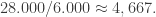
Imagine that there are 1000 projects like this, then this per € 1 risk is equal to approximately , which is a lot lower than the per € 1 risk of approximately that we had in one project. Or in other words, while we expect a € 6.000 gain on average from each project, if we invest in all projects we get a standard deviation for the average gain from all projects of . As zero is more than 6 standard deviations away from 6000, this means that the chances of getting a negative total amount from investing in all these projects is essentially zero.

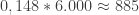
Here is my second attempt to try to convince you that there is essentially zero risk in investing in many independent projects. If you don’t enjoy this probability theory argument, I would recommend you open a spreadsheet such Excel and generate a column of 1000 random numbers that are uniformly distributed between zero and one. In Excel you can do this with the command “rand()”. In the next column you write a 0 for failure if the random number on the left is below 0,2 and 1 otherwise. In Excel you can do this with the command “if(A1<0,2;0;1)” (and pulling this all the way down the column). This means you are generating a Bernoulli random variable (as in my first attempt). In the third column you multiply the entry from the second column with 70.000 and subtract 50.000. Now, in this column, you have the outcome of all 1000 projects. Then in some cell you compute the average payment from all these projects. In Excel this is done with the command “average(C1:C1000)”. Then by pressing space and then enter in an empty cell (or some other activity) you simulate the outcome of these 1000 projects once. Do this over and over and watch the average payment cell. You will see that it varies around € 6000, half the time it is somewhat higher, half the time it is somewhat lower. But no matter how often you try this number is virtually never below zero. In other words we come to the same conclusion as in my probability theory explanation: that there is essentially no risk if you invest in a 1000 such (stochastically independent!) projects.

Because of this, and because big investors do have a lot of money so that they can invest in many projects at the same time, in principle such investors would (in the absence of any better investment opportunities) accept an interest rate for your loan even as low as 12.5% (at which they make on average zero profits) or let’s say they would accept any interest that is at least a little bit above 12.5%.

The actual interest you will get in the end depends on the overall supply and demand of money. See the end of the previous post.